1. DataFrame을 이용한 시각화

import pandas as pd
import numpy as np
import matplotlib.pyplot as plt

# 1. 딕셔너리를 이용한 DataFrame 생성
np.random.seed(100)
data = {'a':np.arange(50),
        'c':np.random.randint(0,50,50),
        'd':np.random.randn(50)
       }

data['b'] = data['a'] + 10 *np.random.randn(50)
data['d'] = np.abs(data['d']) * 

pd.DataFrame(data)


result의 일부


2. 산점도 그래프를 이용한 시각화 .. scatter

산점도 그래프는 scatter() 함수를 사용한다.
X, Y 축에 해당하는 데이터의 상관관계 ... 얼마나 많이 분포 혹은 흩어져 있는지를 한 눈에 확인 가능
X, Y 두 개의 축을 기준으로 데이터가 얼마나 퍼져있는지를 알 수 있다.


plt.scatter([1,2,3,4], [10, 30, 20, 40], s=[100, 200, 350, 500], c=range(4), cmap='jet')  # 구글에서 pyhton cmap 검색해서 튜토리얼
plt.colorbar()  # strong과 color의 맵핑을 해준다
plt.show()


result


plt.scatter('a','b',data=data)
plt.show()


result


# plt.scatter('c','d',data=data, c='c' , s='d')
# scatter 자체는 legend를 사용할 수 없다.

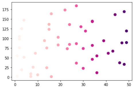
plt.scatter('c','d',data=data, c='c' , s=50, cmap="RdPu")
plt.show()


result


import seaborn as sns

cutoff = (data['a'] > 25) & (data['b'] > 20)

sns.set_style('dark')
data['color'] = np.where(cutoff==True, "red", "blue")
sns.regplot(x = data['a'], 
            y = data['b'],
            scatter_kws={'facecolors' : data['color']}
           )

plt.title("Scatter and Plot", fontsize=16)
plt.show()


result


3. Subplot으로 plot(), scatter(), bar() 동시에 시각화

names = ['group-a', 'group-b', 'group-c']  # X 값으로 이용
values = [1, 10, 100]  # Y 값으로 이용


plt.figure(figsize=(9,3))  # 3등분 하기 쉽도록 전체 영역을 새롭게 잡아놓는다. 
plt.subplot(131)  # 1개를 지정하는 3개 중에 1번째 라는 의미
plt.plot(names, values)

plt.subplot(132)  # 1개를 지정하는 3개 중에 2번째 라는 의미
plt.bar(names, values)

plt.subplot(133)  # 1개를 지정하는 3개 중에 3번째 라는 의미
plt.scatter(names, values)

plt.show()


'데이터과학자 - 강의 > 데이터분석' 카테고리의 다른 글

210728 시각화 : MatPlot - 1  (0) 2021.08.02
210727 pandas의 pivot table  (0) 2021.08.01
210726 pandas의 groupby  (0) 2021.07.27
210723 pandas의 concat, merge  (0) 2021.07.27
210722 pandas의 DataFrame -2, NaN  (0) 2021.07.22

1. MatPlot을 이용한 시각화

파이썬으로 데이터를 시각화하는 데에는 Matplotlib 라이브러리를 가장 많이 사용한다.
Matplotlib 는 파이썬에서 2D 형태의 그래프, 이미지 등을 그릴 때 사용하는 것으로
실제 과학 컴퓨팅 분야나 인공지능 분야에서도 많이 사용된다.

Matplotlib 모듈에는 다양한 모듈들이 많이 있는데 그 중에서 가장 기본이 되는 서브모듈이 pyplot이다.


1-1. plot() : 직선 혹은 꺾은선 그래프를 그릴 때 사용

import matplotlib.pyplot as plt

# 꺾은선 그래프
plt.plot([1,2,3,4],[1,4,9,16], '--')  # plt.plot(x축, y축)
plt.show()

# 직선그래프
plt.plot([10,20,30,40], 'bo')  # plt.plot(x축=y축이라 하나만 넣는다)
plt.show()

# 그래프에 기본적인 옵션 추가하기
plt.plot([1,2,3,4],[1,4,9,16], '-ro')  # 'r', 'g', 'o', 
plt.axis([0,6,0,40])  # 앞에 2개가 x축의 크기, 뒤에 2개가 y축의 크기
plt.title("Graph Test")
plt.show()

-    : 직선으로 연결
--   : 점선으로 연결
o    : 값에 점 찍기
b, r : 컬러


result1
result2
result3


1-2. 겹쳐진 그래프

import numpy as np
np.random.seed(100)

t = np.arange(0, 5, 0.2)
plt.plot(t, t, 'r--')
plt.show()

plt.plot(t, t, 'r--', t, t**2, 's')
plt.show()

plt.plot(t, t, 'r--', t, t**2, 'bs', t, t**3, 'g^')
plt.show()


result1
result2
result3


1-2-1. 겹쳐진 그래프에 옵션 지정하기

plt.plot(t, t, 'r--', label="A")
plt.plot(t, t**2, 'bs', label="B")
plt.plot(t, t**3, 'g^', label="C")

plt.legend()  # 이 부분을 해줘야 label이 표시된다.
plt.title("Wrapped Graph")
plt.xlabel("X Axis")
plt.ylabel("Y Axis")
plt.show()


result


1-3. 파형을 나타내는 그래프

t = np.arange(0,12,0.01)
'''
기본으로 존재하는 figure가 아닌 새로운 figure를 생성하기 위해 다시 영역을 설정한다.
'''

plt.figure(figsize=(15,5))

plt.plot(t, np.sin(t), 'r', lw=13, label="sin") # lw : Line Width
plt.plot(t, np.cos(t), 'b', label="cos")

plt.legend()
plt.grid()

plt.xlabel('time')
plt.ylabel('Amplitude')

plt.title("Graph Test2..")

plt.show()


result


'데이터과학자 - 강의 > 데이터분석' 카테고리의 다른 글

210729 시각화 : MatPlot - 2  (0) 2021.08.06
210727 pandas의 pivot table  (0) 2021.08.01
210726 pandas의 groupby  (0) 2021.07.27
210723 pandas의 concat, merge  (0) 2021.07.27
210722 pandas의 DataFrame -2, NaN  (0) 2021.07.22

1. PivotTables

피벗함수는 DataFrame 의 데이터를 ReShape하는 강력한 방법
여러 컬럼을 index, values, columns 값으로 사용할 수 있다.

import numpy as np
import pandas as pd
from pandas import DataFrame
import matplotlib.pyplot as plt

data = {
    "도시": ["서울", "서울", "서울", "부산", "부산", "부산", "인천", "인천"],
    "연도": ["2015", "2010", "2005", "2015", "2010", "2005", "2015", "2010"],
    "인구": [9904312, 9631482, 9762546, 3448737, 3393191, 3512547, 2890451, 263203],
    "지역": ["수도권", "수도권", "수도권", "경상권", "경상권", "경상권", "수도권", "수도권"]
}

df1 = DataFrame(data)
df1

df1


df1.pivot_table(values='인구', index='도시', columns='연도')
df1.pivot_table(values='인구', index='도시', columns='연도', margins=True)

result : margin=False
result : margin=True

df1.인구.mean()


#result
5350808.625

margin=True 한 결과와 df1.인구.mean() 한 결과가 같다. 즉, pivot_table의 기본 함수는 mean이다.

기본 함수가 mean이라는 것은 다른 함수로 변경이 가능하다.


df1.pivot_table('인구', index=['연도', '도시'])

result

연도별로 그룹핑하고 도시별로 그룹핑을 한 번더 한 자료가 되었다.
pivot_table에서 index는 그룹핑하고 동일하다.


df1.groupby(by=['연도', '도시']).mean()

result

'데이터과학자 - 강의 > 데이터분석' 카테고리의 다른 글

210729 시각화 : MatPlot - 2  (0) 2021.08.06
210728 시각화 : MatPlot - 1  (0) 2021.08.02
210726 pandas의 groupby  (0) 2021.07.27
210723 pandas의 concat, merge  (0) 2021.07.27
210722 pandas의 DataFrame -2, NaN  (0) 2021.07.22

DataFrame - 데이터 그룹핑하기(그룹연산)

통계자료에서 많이 사용한다.
그룹핑 시켜서 합을 도출하거나 혹은 평균값을 구하거나 ... 등등


import numpy as np
import pandas as pd
from pandas import DataFrame
import matplotlib.pyplot as plt

np.random.seed(100)
df = DataFrame({
    'Gender' : ['Female', 'Male', 'Female', 'Male', 'Female', 'Male', 'Female', 'Female'],
    'Smoking' : ['Smoker', 'Smoker', 'Smoker', 'Non-Smoker', 'Non-Smoker', 'Non-Smoker', 'Non-Smoker', 'Smoker'],
    'JumpHeight' : np.random.randint(10, 100, 8),
    'LungCapa' : np.random.randint(10, 100, 8)
})

df


그룹핑 ... groupby()

df.groupby('Gender')


# result
<pandas.core.groupby.generic.DataFrameGroupBy object at 0x000001EE5BBFDEB0>


gropyby()를 하면 그룹핑이 된다. 
근데 눈에 결과가 보이는건 아니고 그룹핑된 객체가 리턴됨.
객체 자체로는 아무것도 못함
객체에 집계함수, 통계함수를 적용해야 눈으로 보이는 결과가 나옴

groupby 함수로 데이터를 그룹핑하면 DataFrameGroupBy 객체가 리턴된다.
이 상태로는 아무것도 못함...여기에 통계함수를 적용해야 한다.


df.groupby('Gender').sum()

result

결과에 smoking이 나오지 않았는데 Numeric한 데이터가 아니라 그렇다


성별로 나누고 다시 흡연여부로 나눔 ,,, sum()적용

df.groupby(['Gender', 'Smoking']).sum()


result


특정한 컬럼값에 대해서만 그룹핑하고 싶다면?

df.groupby('Gender')['LungCapa'].max()
df.groupby('Gender')['LungCapa'].agg('max')  # 동일한 결과


#result
Gender
Female    70
Male      76
Name: LungCapa, dtype: int32

특정한 컬럼에 대해서 그룹핑하면 ... 시리즈를 반환한다


df.groupby('Gender')[['LungCapa']].max()
df.groupby('Gender')[['LungCapa']].agg('max')  # 대괄호를 하나 더 감싸주면 DF로 반환됨 - result1
df.groupby('Gender')['LungCapa'].agg(['max'])  # 결과는 같은데 컬럼명이 바뀌네? - result2

result1
result2


agg는 aggregation 의 약어로 여러 개의 함수를 동시에 사용해서 그룹핑이 가능하다.

df.groupby('Gender')['LungCapa'].agg(['sum', 'max', 'min', 'count'])

result


알아두어야 할 함수

  • unique - DISTINCT
  • describe - 4분위 함수
  • value_counts - 해당 컬럼에서 그 값이 몇 번 나왔는지 확인 가능. 빈도수 확인하는 함수
  • apply - pandas에서 내가 직접 함수를 정의할 때 적용

df


1. unique()

df['Gender'].unique()


#result
array(['Female', 'Male'], dtype=object)

2. describe() : 데이터에 대한 간단한 설명 ==> 간단한 통계

df.describe()

result


3. value_counts()

빈도수 확인 ... 해당 컬럼에서 특정 값이 몇 번 나왔는지

df['Smoking'].value_counts()


#result
Non-Smoker    4
Smoker        4
Name: Smoking, dtype: int64

4. apply()

판다스에서는 여러가지 통계함수를 제공하고 있지만...
내가 직접 함수를 정의해서 사용해야 하는 경우가 발생한다.
사용자정의 함수 ..

이렇게 만든 함수를 가져다 사용할 때 apply를 적용함


def add(x):
    return x + 12

df[['LungCapa']].apply(add)
df[['LungCapa']].agg(add)  # 사실 agg도 되기 때문에 agg가 활용도가 높다.

'데이터과학자 - 강의 > 데이터분석' 카테고리의 다른 글

210728 시각화 : MatPlot - 1  (0) 2021.08.02
210727 pandas의 pivot table  (0) 2021.08.01
210723 pandas의 concat, merge  (0) 2021.07.27
210722 pandas의 DataFrame -2, NaN  (0) 2021.07.22
210721 pandas의 DataFrame  (0) 2021.07.22

DataFrame - 데이터 병합

  • Concat
    단순히 하나의 DataFrame에 다른 DataFrame을 연속적으로 붙이는 방법
    이 경우에는 두 DataFrame이 서로 동일한 인덱스, 컬럼을 가지고 있는 경우가 대부분이다
    위, 아래로 연결되는 방식이 기본이지만 좌, 우 연결도 가능하다
    outer join이 기본으로 동작
    key를 이용해 Concat을 활용해서 사용한다.

  • Merge

1. pandas의 concat

import numpy as np
import pandas as pd
from pandas import DataFrame, Series
import matplotlib.pyplot as plt

df1 = DataFrame({
    'A':['A0','A1','A2','A3'],
    'B':['B0','B1','B2','B3'],
    'C':['C0','C1','C2','C3'],
    'D':['D0','D1','D2','D3'],    
})

df2 = pd.DataFrame({
    'A':['A4', 'A5', 'A6', 'A7'],
    'B':['B4', 'B5', 'B6', 'B7'],
    'C':['C4', 'C5', 'C6', 'C7'],
    'D':['D4', 'D5', 'D6', 'D7'],
})

df1
df2


df1, df2 데이터를 가만히 봐보자
어떻게 병합하는게 좋을까?
    ==> 상하 연결
    ==> pandas에서 제공하는 함수 concat()
::
결과를 확인하면
0123, 0123 동일한 인덱스 값이 그대로 반복된다.
ignore_index = True 옵션을 지정한다.


# result1 = pd.concat([df1, df2])
result1 = pd.concat([df1, df2], ignore_index=True)
result1


좌우 병합은?
ignore_index=True 이거하면 해당 컬럼명이 인덱스로 대체된다
result2 = pd.concat([df1, df2], axis=1)  # 행이 아닌 열로 합쳐진다.


result2 = pd.concat([df1, df2], axis=1, ignore_index=True)
result2


1-1. KEYS

각각 다른 데이터를 병합하는 것이니 출처를 표기해준다. ex)2020년 데이터 or 2021년 데이터
그룹핑, 세분화하는데 쓰인다

result2 = pd.concat([df1, df2], keys=['Female', 'Male'])  # ignore_index=True 랑은 중복이 안되네
result2


df3 = DataFrame({
    'A':['A0','A1','A2','A3'],
    'B':['B0','B1','B2','B3'],
    'C':['C0','C1','C2','C3']      
})

df4 = pd.DataFrame({
    'A':['A4', 'A5', 'A6', 'A7'],
    'B':['B4', 'B5', 'B6', 'B7'],
    'C':['C4', 'C5', 'C6', 'C7'],
    'D':['D4', 'D5', 'D6', 'D7'],
})

df3
df4


위 df3, df4 데이터는 행과 열 인덱스가 일치하지 않는 데이터프레임이다.
axis=0 을 기준으로 병합하기 때문에 concat은 상하로 데이터를 이어붙이게 될 것이다.
어떤 현상이 발생할까?
outer join이기 때문에 없는 부분을 NaN으로 채운다.


result3 = pd.concat([df3, df4], ignore_index=True)  # join='outer' 가 default
result3

# 둘 다 공통적으로 가지고있는 열만 가지고 온다.
result4 = pd.concat([df3, df4], ignore_index=True, join='inner')
result4


2. pandas의 merge

df1, df2는 인덱스만 다르고 모든 값을 동일하게 가지고 있다.
df3는 Color_num라는 다른 column을 가지고 있다.

df1 = DataFrame({ 'Year':[2001,2002,2003,2004],
                  'Product_Code':[11,22,33,44],
                  'Price':[10000,20000,30000,40000]},
                   index=list('1234'))

df2 = DataFrame({ 'Year':[2001,2002,2003,2004],
                  'Product_Code':[11,22,33,44],
                  'Price':[10000,20000,30000,40000]},
                   index=list('5678'))

df3 = DataFrame({ 'Year':[2001,2003,2004,2005],
                  'Product_Code':[11,22,33,44],
                  'Color_num':[33,44,55,99]},
                   index=list('1234'))

df1
df2
df3


df1, df2를 merge
1. 표현법이 concat과 다르다 ... [ ] 들어가지 않는다...
2. 인덱스와 상관없이 병합되고(*좌우병합이기 때문) 값이 같다면 중복표기되지 않는다.


result01 = pd.merge(df1, df2)
result01


df1_1 = DataFrame({ 'Year':[2001,2002,2003,2004],
                  'Product_Code':[11,22,33,44],
                  'Price':[15000,25000,35000,45000]},
                   index=list('1234'))

df1_1


df1_1 와 df1을 merge.... on을 사용하지 않으면 아무것도 나오지 않는다.

병합할 때의 기준이 되는 컬럼을 지정하는 것이 on이다
기준이 되는 컬럼 외에는 다 중복으로 데이터가 표기된다.

result02_1 = pd.merge(df1, df1_1), on=['Year']
result02_1

result02_2 = pd.merge(df1, df1_1, on=['Year'])
result02_2

result02_1
result02_2

result03 = pd.merge(df1, df1_1, on=['Year', 'Product_Code'])
result03


3. set_index()

특정한 컬럼을 인덱스로 지정함으로써
DataFrame을 좀 더 깔끔하고 직관적으로 볼 수 있다.

result03.set_index('Year', inplace=True)
result03


4. df1, df3 merge 

df1
df3

how 옵션이 있다... 어떻게 merge 할 것인가? concat의 join= 과 같다
여기서 inner가 dafault 이다.

result05 = pd.merge(df1, df3, how='outer', on='Year')
result05


매개변수 중 left(df1)의 Year의 모든 값을 살리면서 join

result06 = pd.merge(df1, df3, 'left', on='Year')
result06

'데이터과학자 - 강의 > 데이터분석' 카테고리의 다른 글

210727 pandas의 pivot table  (0) 2021.08.01
210726 pandas의 groupby  (0) 2021.07.27
210722 pandas의 DataFrame -2, NaN  (0) 2021.07.22
210721 pandas의 DataFrame  (0) 2021.07.22
210721 numpy.ndarray-2, pandas.Series  (0) 2021.07.21

1. DataFrame - 데이터 검색하기

  • iloc
  • loc
  • at
  • iat

    i가 붙은 친구들은 정수 index로 검색하고 없는 친구들은 label로 검색한다.


df1

1-1. iloc, loc

# 2, 3번째 줄의 데이터를 iloc, loc로 가져와보자
print(df1.iloc[1:3, 0:4])  # 마지막 숫자는 미만인것도 똑같다.
print('=' * 50)
print(df1.iloc[1:3, :])  # 결과 같음
print('=' * 50)
print(df1.iloc[1:3])  # 결과 같음
print('=' * 50)
print('=' * 50)
print(df1.loc[1:2])  # 결과 같음. 그렇지만 iloc는 마지막값 미만이지만 loc는 마지막값이 포함이다
print('=' * 50)
print(df1.loc[1:2, 'name':'phone']) 


#result
     name   addr  age  phone
1   Peter  TEXAS   44    NaN
2  Tomhas     LA   55    NaN
==================================================
     name   addr  age  phone
1   Peter  TEXAS   44    NaN
2  Tomhas     LA   55    NaN
==================================================
     name   addr  age  phone
1   Peter  TEXAS   44    NaN
2  Tomhas     LA   55    NaN
==================================================
==================================================
     name   addr  age  phone
1   Peter  TEXAS   44    NaN
2  Tomhas     LA   55    NaN
==================================================
     name   addr  age  phone
1   Peter  TEXAS   44    NaN
2  Tomhas     LA   55    NaN


1-2. iat, at

# 스칼라값 가져오기.. iat, at
print(df1.iloc[1:3])
print(df1.loc[1:2])
print('=' * 50)

# 토마스의 나이 55를 출력
# 로버트의 주소 TEXAS를 출력
print(df1.iat[2,2])
print(df1.iat[3,1])
print('=' * 50)
print(df1.at[2, 'age'])
print(df1.at[3, 'addr'])

# iat를 이용해서 토마스의 나이를 50세로 변경
'''
지금과 같은 경우가 단독 스칼라값을 검색해야하는 때이고
이럴 때 iat를 많이 사용한다.
ex) 특정한 값을 찾아서 값을 변경한다
'''
df1.iat[2,2] = 50
df1


#result
     name   addr  age  phone
1   Peter  TEXAS   44    NaN
2  Tomhas     LA   55    NaN
     name   addr  age  phone
1   Peter  TEXAS   44    NaN
2  Tomhas     LA   55    NaN
==================================================
55
TEXAS
==================================================
55
TEXAS

df1.iat[2,2] = 50 결과


2. 데이터 삭제하기 - 누락데이터 정책

  • drop() ()안에 라벨명을 넣어야한다. default로 원본이 변경되지 않고(inplace=false) 행기준(axis=0)으로 설정되어 있다.
  • n개 이상일 때만 삭제
  • fillna(0) - mean, max, min 값으로 변경 등
# 5번째 row를 추가 ... loc를 이용해서 ... 값은 전부 누락데이터로 추가해라
df1.loc[4] = np.nan
df1

df1.loc[4] = np.nan 결과

# phone에 해당하는 부분을 삭제하고 원본 반영
df1.drop('phone', axis=1, inplace=True)
df1

df1.drop('phone', axis=1, inplace=True) 결과

values를 삭제하는 작업은 기본적으로 원본 데이터에 반영되지 않는다.

이를 원본 데이터에 반영하기 위해 inplace=True 매개변수를 추가한다.


3. DataFrame - 데이터 정렬하기

  • sort_index()
  • sort_values()

df2

3-1. sort_index()

df2.sort_index(axis=1, ascending=False)  # oracle의 orderby랑 같은 기능

결과


3-2. sort_values()

df2.sort_values(by=['four'])

결과


  • unique() : 중복된 값을 배제하는 기능. 오라클의 Distinct
  • value_counts() : value의 개수를 세주는 함수
  • isin() : 특정한 데이터가 들어있는지 여부를 판단하는 함수
# df3['day']  # 이 방법으로 하면 다나와서 안된다
df3['day'].unique()


#result
['Sun', 'Sat', 'Thur', 'Fri', nan], dtype=object
df3['day'].value_counts()  # 누락 데이터는 통계함수, count함수에서 제외된다.


#result
Sat     87
Sun     76
Thur    62
Fri     19
Name: day, dtype: int64
df3['day'].isin(['Sat', 'Sun'])


#result
0       True
1       True
2       True
3       True
4       True
       ...  
240     True
241     True
242     True
243    False
244    False
Name: day, Length: 245, dtype: bool

DataFrame - 누락데이터 처리하기

데이터 분석시 제공된 데이터를 살펴보면 값이 입력되어 있지 않은 경우가 종종 있다.
이런 경우를 Missing Value 가 있다고 표현한다.

<<< Missing Value 를 처리하는 대표적인 전략 >>>

  • 데이터가 거의 없는 Feature는 Feature 자체를 Drop 시킨다
  • 데이터가 없으면 바로 Drop
  • Missing Value의 최소 개수를 정해서 어느 이상의 개수를 넘어서면 Drop
  • 최빈값, 평균값, 0 등의 값으로 비어있는 데이터를 채우기

    pandas는 누락된 데이터를 모두 NaN으로 처리한다.
    또한 판다스 객체의 모든 통계함수는 누락 데이터를 무시하고 연산을 진행한다.

    <<< 누락 데이터를 처리하는 함수들 >>>
  • dropna() -- NaN이 하나라도 있는 row는 모두 삭제. default가 how='any'임 3번이랑 같음
  • dropna(how='all') -- 모든 값이 NaN인 경우만 삭제
  • dropna(how='any') -- NaN이 하나라도 있는 row는 모두 삭제
  • dropna(thresh=3) -- 일반 데이터의 개수가 thresh값 보다 많으면 생존 아니면 삭제
  • fillna()
  • isnull()
  • notnull()
import numpy as np
import pandas as pd
from pandas import DataFrame
from numpy import nan as NA

df = DataFrame([[1, 6.5, 3],
               [1, NA, NA],
               [NA, NA, NA],
               [NA, 6.7, 2]
               ])
df

removeNA = df.dropna()  # 이런 드랍이나 삭제같은 친구들은 원본을 절대 건드리지 않는다.
                        # 누락 데이터가 하나라도 있으면 해당 row가 삭제된다.
removeNA


df.dropna(how='all')


df.dropna(thresh=2)  # thresh는 역치값 임계치값 thresh는 NaN의 개수가 아니다 일반 데이터의 개수이다.
df.dropna(thresh=3)  # thresh=3을 해보면 확실하다.

thresh=2
thresh=3


누락 데이터 채우기

df.fillna(0)
df.fillna(df.mean())  # 각 Series의 평균을 넣는듯
df.fillna(value=5)
df.fillna(method='ffill')  # NaN 바로 위에 있는 값으로 채운다

df.fillna(0)
df.fillna(df.mean())
df.fillna(value=5)
df.fillna(method='ffill')

1. DataFrame 생성

    DataFrame은 2차원 배열 형식
    표같은 스프레드 시트 자료구조
    여러 개의 column을 가지며 서로 다른 종류의 값(?)이 담긴다.


DataFrame 생성하는 방법

  • 리스트 값을 딕셔너리로 사용
  • Numpy 배열을 이용
  • read_csv(), read_excel()... 등 함수 사용

1-1. 딕셔너리로 DataFrame 생성 - 자주 사용

import numpy as np
import pandas as pd
from pandas import DataFrame, Series
import matplotlib.pyplot as plt

'''
자주 사용하는 이유
DataFrame 생성할 때 명시적으로 column을 주지 않아도
딕셔너리의 key 값을 column으로 가져오기 때문
'''
dic = {'state' : ['Ohio', 'Ohio', 'Ohio', 'Nevada', 'Nevada', 'Nevada'],
        'year' : [2000, 2001, 2002, 2001, 2002, 2003],
         'pop' : [1.5, 1.7, 3.6, 2.4, 2.9, 3.2]
      }

dic_df = DataFrame(dic)
dic_df

print(dic_df.state)
print(type(dic_df.state))
print('=' * 100)

print(dic_df.state)
print(type(dic_df.year))
print('=' * 100)

# print(dic_df.pop)  <== 이대로 작성하면 내장함수 pop이 우선적으로 나와 class method로 나온다
print(dic_df['pop'])
print(type(dic_df['pop']))


#result
0      Ohio
1      Ohio
2      Ohio
3    Nevada
4    Nevada
5    Nevada
Name: state, dtype: object
<class 'pandas.core.series.Series'>
====================================================================================================
0      Ohio
1      Ohio
2      Ohio
3    Nevada
4    Nevada
5    Nevada
Name: state, dtype: object
<class 'pandas.core.series.Series'>
====================================================================================================
0    1.5
1    1.7
2    3.6
3    2.4
4    2.9
5    3.2
Name: pop, dtype: float64
<class 'pandas.core.series.Series'>


DataFrame은 여러 개의 컬럼을 가지면서
서로 다른 종류의 값이 담긴다.

DataFrame은 여러 개의 Series의 결합체다.
Series는 ndarray 클래스 타입으로 동일한 자료형을 가진다.
각각의 Series가 다른 dtype을 가져도 DataFrame으로 묶을 수 있다.

dic_df 결과


data1 = {
    'name' : ['James', 'Peter', 'Tomhas', 'Robert'],
    'address' : ['NY', 'TEXAS', 'LA', 'TEXAS'],
    'age' : [33, 44, 55, 66]    
}

df1 = DataFrame(data1)
df1


df1 결과

print(df1.T) # ==> 행과 열을 바꿔준다.


#result
             0      1       2       3
name     James  Peter  Tomhas  Robert
address     NY  TEXAS      LA   TEXAS
age         33     44      55      66

1-2. Numpy배열 데이터로 생성

# 위치 매개변수와 키워드 매개변수를 사용
np.random.seed(100)
df2 = DataFrame(np.random.randint(10, 100, 16).reshape(4, 4), 
                    index=list('abcd'),
                    columns=list('abcd')
               )

# column명을 수정
df2.columns = ['one', 'two', 'three', 'four']  # column명을 한 번에 수정할 때 사용
df2

df2의 결과 column이 바뀐 상태


1-3. read_csv() 함수로 생성

csv 파일을 읽어들여서 생성


df3 = pd.read_csv('../data/tips.csv')  # 폴더에 kaggle에서 받아온 자료가 있음.
df3


2. DataFrame 구조

구조를 확인하는 속성

  • index
  • columns
  • values
  • dtypes
  • info()
  • shape

print(df3.index)
print()
print(df3.columns)
print()
print(df3.values)
print()
print(df3.dtypes)
print()
print(df3.shape)  # 튜플 형식으로 출력


#result
RangeIndex(start=0, stop=245, step=1)

Index(['total_bill', 'tip', 'sex', 'smoker', 'day', 'time', 'size'], dtype='object')

[[16.99 1.01 'Female' ... 'Sun' 'Dinner' 2.0]
 [10.34 1.66 'Male' ... 'Sun' 'Dinner' 3.0]
 [21.01 3.5 'Male' ... 'Sun' 'Dinner' 3.0]
 ...
 [17.82 1.75 'Male' ... 'Sat' 'Dinner' 2.0]
 [18.78 3.0 'Female' ... 'Thur' 'Dinner' 2.0]
 [25.34 nan nan ... nan nan nan]]

total_bill    float64
tip           float64
sex            object
smoker         object
day            object
time           object
size          float64
dtype: object

(245, 7)


df3.info()  # 각 column의 dtype과 누락데이터의 여부를 확인 가능


#result
<class 'pandas.core.frame.DataFrame'>
RangeIndex: 245 entries, 0 to 244
Data columns (total 7 columns):
 #   Column      Non-Null Count  Dtype  
---  ------      --------------  -----  
 0   total_bill  245 non-null    float64
 1   tip         244 non-null    float64
 2   sex         244 non-null    object 
 3   smoker      244 non-null    object 
 4   day         244 non-null    object 
 5   time        244 non-null    object 
 6   size        244 non-null    float64
dtypes: float64(3), object(4)
memory usage: 13.5+ KB


조회를 확인하는 함수

  • info()
  • head()
  • tail()
df3
df3.head()  # 위에서부터 추출 조회. default는 5
df3.head(10)

df3.tail()
df3.tail(10)

df3.tail(10)의 결과


3. DataFrame - 컬럼명 변경 및 추가하기

원본이 바로 변경되는 옵션과 원본이 변경되지 않는 옵션이 존재한다.

1) 컬럼명 전체 수정 ... columns => 원본 바로 변경
2) 컬럼명 부분 수정 ... rename => 원본 변경 안됨

:: 원본 데이터를 변경하려면 새로운 옵션을 하나 익혀야 한다.
inplace=True 추가해야 한다.

df2

# 1. 컬럼명 변경하기
df2.columns = ['A-class', 'B-class', 'C-class', 'D-class']
df2


df1
df1.rename(columns={'address' : 'addr'}, inplace=True)

df1


컬럼 추가하기

df1
df1['phone'] = np.nan

df1


1. ndarray의 인덱싱과 슬라이싱

# 1) 2차원 arr4에서 18을 뽑아봐라
'''
2차원 배열의 인덱스는 [   ,   ]
콤마를 기준으로 2개의 인자를 받음
앞 인자값은 행의 index, 뒤 인자값은 열의 index
만약에 :넣으면 모든 요소에 해당된다.
'''
print(arr4[0, 2])  # arr4[0][2]

# 2) 2번째 라인 [13, 13, 13, 17] 값을 가져오려면?
print(arr4[1, :])
print(arr4[1:2, :])  # 2차원으로 출력된다.

# 3) 전체 행에 대해서 4번째 열을 다 가지고 와보자
print(arr4[:, 3])  # 이렇게하면 1차원 배열로 가지고온다
print(arr4[:, 3:])  # 이렇게하면 2차원 배열로 가지고온다

# 4) 전체 행에 대해서 1,2 열을 가지고 와보자
print(arr4[:, :2])


#result
18
====================================================================================================
[13 13 13 17]
[[13 13 13 17]]
====================================================================================================
[11 17 19 13]
[[11]
 [17]
 [19]
 [13]]
====================================================================================================
[[12 13]
 [13 13]
 [10 11]
 [10 14]]

2. Numpy 통계함수
    Pandas에서 디테일하게 다루기 때문에 간단하게 정리만 함
    sum, mean, std, min, max, argmax, argmin, cunsum
      - mean : 평균
      - argmax : max 값의 index 값
      - argmin : min 값의 index 값
      - cunsum : 누적 합계


x = np.array([[1, 2], [3, 4]])
print(x)
print('=' * 50)
print(np.sum(x))
# axis 는 축 axis=0 은 행기준, axis=1 은 열기준
'''
행기준 : 모든 행을 더해야 한다 => 각 열에 대한 합을 연산
열기준 : 모든 열을 더해야 한다 => 각 행에 대한 합을 연산
'''
print(np.sum(x, axis=0))  
print(np.sum(x, axis=1))


#result
[[1 2]
 [3 4]]
==================================================
10
[4 6]
[3 7]


print(arr4)
print('=' * 100)
print(np.sum(arr4))
print(np.sum(arr4, axis=1))
print(np.sum(arr4, axis=0))
print('=' * 100)
print(np.cumsum(arr4))
print(np.cumsum(arr4, axis=1))
print(np.cumsum(arr4, axis=0))
print('=' * 100)
print(np.argmax(arr4, axis=0))


#result
[[12 13 18 11]
 [13 13 13 17]
 [10 11 19 19]
 [10 14 17 13]]
====================================================================================================
223
[54 56 59 54]
[45 51 67 60]
====================================================================================================
[ 12  25  43  54  67  80  93 110 120 131 150 169 179 193 210 223]
[[12 25 43 54]
 [13 26 39 56]
 [10 21 40 59]
 [10 24 41 54]]
[[12 13 18 11]
 [25 26 31 28]
 [35 37 50 47]
 [45 51 67 60]]
====================================================================================================
[1 3 2 2]

3. Pandas의 Series

Series

Pandas는 Panel Datas의 약자로 파이썬을 이용한 데이터 분석에서 가장 많이 사용되는 라이브러리
Numpy 기반으로 만들어졌으며 데이터 분석을 하기위한 효율적인 구조를 제공한다.

Pandas의 자료구조

  • Series : 1차원 배열형태의 데이터 구조를 가진다. (벡터)
    별도로 행을 지정해주지 않으면 인덱스는 리스트처럼 정수로 설정
  • DataFrame : 2차원 배열 형태의 데이터 구조를 가진다. - 가장 많이 사용 (매트릭스)
    행을 구분하는 index와 열을 구분하는 column이 있다. 별도로 행과 열을 지정해주지 않으면 인덱스는 리스트처럼 정수로 설정

3-1. 시리즈 생성, 구조확인

import numpy as np
import pandas as pd
from pandas import Series, DataFrame

# 시리즈 구조를 먼저 확인
'''
data
index로 구성된다.
columns 옵션은 빠져있다.
이유는 벡터구조이기 때문이다.
'''

np.random.seed(100)
'''
인덱스를 명시적으로 지정하지 않으면
자동적으로 0 ~ N-1 까지의 정수로 잡힌다.

인덱스를 명시적으로 지정할 때는
반드시 리스트 형태의 값으로 지정한다.
'''
ser1 = Series(np.random.randint(10, 20, 5))
print(ser1)


#result
0    18
1    18
2    13
3    17
4    17
dtype: int32


np.random.seed(100)
ser1 = Series(np.random.randint(10, 20, 5), index=list('abcde'))
print(ser1)
print('*' * 100)
print(ser1.index)
print('*' * 100)
print(ser1.values)
print('*' * 100)
print(ser1.dtype)


#result
a    18
b    18
c    13
d    17
e    17
dtype: int32
****************************************************************************************************
Index(['a', 'b', 'c', 'd', 'e'], dtype='object')
****************************************************************************************************
[18 18 13 17 17]
****************************************************************************************************
int32


3-2. 시리즈 값 조회하기

슬라이싱 방법

1) 숫자사용 : 마지막 숫자는 포함 안됨
2) 라벨사용 : 마지막 라벨은 포함됨


ser1['c']  # 같은 결과
ser1[2]  # 같은 결과

print(ser1[1:4])
print(ser1['b':'d'])

#응용해서 조회해보자
ser1
ser1_1 = ser1[::2]
print('*' * 100)
print(ser1_1)


#result
b    18
c    13
d    17
dtype: int32

b    18
c    13
d    17
dtype: int32
****************************************************************************************************
a    18
c    13
e    17
dtype: int32


3-3. 시리즈간의 연산

'''
NaN : 누락데이터, 결측값이라고 함. NaN의 dtype은 float64이다.
ser1에는 b와 d에 값이 있지만 ser1_1에는 없기때문에 더했을 때 NaN값이 나온다.

연산결과 dtype int32에서 float64로 변경되었다. NaN의 dtype이 float64이기 때문
그럼 왜 제대로 연산된 a, c, e 까지 float64로 변경되었는가?
pandas의 Series는 ndarray 타입이기 때문에 dtype이 통일되어야 하기 때문이다.
'''
print(ser1)
print(ser1_1)
print('='*100)

resultSer = ser1 + ser1_1
print(resultSer)


#result
a    18
b    18
c    13
d    17
e    17
dtype: int32

a    18
c    13
e    17
dtype: int32
====================================================================================================
a    36.0
b     NaN
c    26.0
d     NaN
e    34.0
dtype: float64


3-4. 누락 데이터 조회하기

  • isnull()
  • notnull()
resultSer
print(resultSer.isnull())
print()
print(resultSer.notnull())
print()
print(resultSer.isnull().sum())
print('=' * 100)
print(resultSer[resultSer.isnull()])
print()
print(resultSer[resultSer.notnull()])


#result
a    False
b     True
c    False
d     True
e    False
dtype: bool

a     True
b    False
c     True
d    False
e     True
dtype: bool

2
====================================================================================================
b   NaN
d   NaN
dtype: float64

a    36.0
c    26.0
e    34.0
dtype: float64


오늘부터 본격적으로 데이터분석, 딥러닝, 머신러닝 수업에 들어간다.

그 시작으로 필요한 설치를 진행했다.


============================================================================

1. Anaconda 설치

1-1. Anaconda 설치 파일 다운로드

https://www.anaconda.com/products/individual

아나콘다 홈페이지의 메인 페이지 하단에서 운영체제에 맞는 설치 파일 다운


1-2 설치 진행

설치 파일을 우클릭 - 관리자 권한으로 실행하여 설치를 진행한다. 

상단 이미지처럼 권한만 Just Me와 경로만 원하는 경로로 변경하고 default설치를 진행했다.


============================================================================

2. jupyter 실행 설정

2-1. 바탕화면에 바로가기 생성

윈도우 메뉴를 실행해보면 Anaconda가 설치되어 올라온다.

Jupyter Notebook을 그대로 드래그해 바탕화면에 바로가기를 생성한다.


2-2. 바로가기 속성 변경

우클릭 ㅡ 속성에 들어가면 해당화면이 바로뜬다. 여기서 " " 안이 다른 내용으로 채워져 있는데

주 작업경로로 변경해주고 실행하면 된다.


============================================================================3. Numpy 배열 생성하기

Numpy는 Numeric Python의 줄임말
수학분야와 관련된 통계, 연산 작업시에 필요한 라이브러리
과학 계산 컴퓨팅과 데이터 분석에 필요한 가장 기본적인 패키지


Numpy배열은 리스트와 거의 흡사하지만

연산 속도가 빠르고 메모리 효율성이 높아서 대용량 데이터를 다루는데 성능상 우위에 있다.


사용하기 전에 라이브러리 모듈을 import 해야 한다.

1) array() 사용
2) random 랜덤함수 사용


3-1. 리스트와 numpy배열을 각각 생성해 두 개를 비교해보자
1.
리스트는 출력 결과가 [ ]안에 들어오고 각 요소들이 ,로 구분된다.
np배열은 출력 결과가 [ ]안에 들어오고 각 요소들이 그냥 나열된다.

2.
np배열의 타입은 ndarray타입 = ndarray 클래스 : 다차원 행렬구조를 지원하는 Numpy의 핵심 클래스


3.

리스트는 원본이 안바뀐다. 원본을 카피해서 새로운걸 만든다.
np배열은 원본뷰가 바뀐다.

메모리 활용적인 성능면에서는 np배열이 성능이 좋아진다.

import numpy as np

myList = [4,5,6,7]

myArr = np.array(myList)

print(myList)
print(myArr)

print(type(myList))
print(type(myArr))
# ========================================================================
list_sub = myList[1:3]  # 슬라이싱(숫자일 때는 뒷 부분 숫자가 포함되지 않는다)
print(list_sub)

arr_sub = myArr[1:3]
print(arr_sub)

list_sub[0] = -5
arr_sub[0] = -5

print(list_sub)
print(arr_sub)
# ========================================================================
print(myList)
print(myArr)


# result==================================================================
[4, 5, 6, 7]
[4 5 6 7]
<class 'list'>
<class 'numpy.ndarray'>
# ========================================================================
[5, 6]
[5 6]
[-5, 6]
[-5  6]
# ========================================================================
[4, 5, 6, 7]
[ 4 -5  6  7]


3-2. random 함수 사용

a = np.random.rand(5)
print(a)
print(type(a))

b = np.random.randint(1,10,5)
print(b)

c = np.random.randn(10)  # 가우시안 표준분포 값
print(c)

# result =================================================
[0.11422413 0.52544893 0.18869529 0.45081129 0.04235887]
<class 'numpy.ndarray'>
[7 1 1 4 6]
[ 2.12486086 -0.21495564  0.65277968 -0.17930631  1.42798995 
 -1.80503814 -0.14268248  0.58640306 -2.55503308 -1.37679103]


3-3. np배열 생성과 동시에 초기화
zeros(), ones(), arange() 함수 사용

# 0으로 초기화
# 0값으로 이뤄진 크기가 10인 배열 생성
# 기본이 실수형이다
az = np.zeros(10)
print(az)
print(type(az))

# 1값으로 이뤄진 크기가 10인 배열 생성
ao = np.ones(10)
print(ao)

# 5값으로 이뤄진 크기가 10인 배열 생성
az5 = np.zeros(10) + 5
print(az5)
ao5 = np.ones(10) * 5
print(ao5)

# eye()
ae = np.eye(3)
print(ae)

# arange()
print(np.arange(3))
print(np.arange(3, 7))
print(np.arange(3, 10 ,2))

# full()
afull = np.full((5, 5), -11)
print(afull)


# result ===============================================================
[0. 0. 0. 0. 0. 0. 0. 0. 0. 0.]
<class 'numpy.ndarray'>
[1. 1. 1. 1. 1. 1. 1. 1. 1. 1.]
[5. 5. 5. 5. 5. 5. 5. 5. 5. 5.]
[5. 5. 5. 5. 5. 5. 5. 5. 5. 5.]
[[1. 0. 0.]
 [0. 1. 0.]
 [0. 0. 1.]]
[0 1 2]
[3 4 5 6]
[3 5 7 9]
[[-11 -11 -11 -11 -11]
 [-11 -11 -11 -11 -11]
 [-11 -11 -11 -11 -11]
 [-11 -11 -11 -11 -11]
 [-11 -11 -11 -11 -11]]


============================================================================

4. Numpy 배열의 속성과 함수

리스트는 여러가지 자료형 저장이 가능하다.
np배열은 하나의 자료형만 저장할 수 있다.

만약에
숫자와 문자가 동시에 저장된다면
capacity가 더 큰 문자로 변환되어서 저장된다.

np배열은 이러한 제약(동일한 datatype만 저장가능)을 가지는 대신에
내부 원소에 대한 접근과 반복문 실행이 빨라지도록 설계되어져 있다.

값의 타입을 지정해서 저장할 때는 dtype 속성을 사용해서 저장한다.
int32, int64, float32, float64 등 지정 가능


import  numpy as np

myList = [1, 2, 3, '4', 5, 6]
print(myList)
print(type(myList))

myArr = np.array([1, 2, 3, '4', 5])
print(myArr)
print(type(myArr))

myArr2 = np.array([1, 2, 3, 4.0, 5])
print(myArr2)
print(type(myArr2))

# myArr3 = np.array([1,2,3,4], dtype='float')
myArr3 = np.array([1,2,3,4], dtype=np.float64)
print(myArr3)
print(type(myArr3))


# result ==============================================================
[1, 2, 3, '4', 5, 6]
<class 'list'>
['1' '2' '3' '4' '5']
<class 'numpy.ndarray'>
[1. 2. 3. 4. 5.]
<class 'numpy.ndarray'>
[1. 2. 3. 4.]
<class 'numpy.ndarray'>


  • ndim, shape, reshape, size, type, dtype
  • Numpy배열의 타입은 ndarray 클래스이다.
    클래스는 다양한 field와 method를 가지고 있고
    ndim, shape, size, dtype은 필드로도 메소드로도 사용가능하다.
    reshape, type은 메소드로만 사용 가능


print(myArr)
print(np.ndim(myArr))  # 몇 차원인지 리턴
print(np.shape(myArr))  # 몇 행, 몇 렬인지 알 수 있다.
print(np.size(myArr))  # 요소의 개수를 리턴
print(type(myArr))

print('*' * 30)

print(myArr.ndim)
print(myArr.shape)
print(myArr.size)
print(myArr.dtype)

print('*' * 30)
# np배열의 원소 값의 타입을 한 번에 바꿀 수 있다. astype()
# astype(), type(), dtype 각각 구분해서 적용할 수 있어야 한다.
myArr_1 = myArr.astype(np.float64)
print(myArr_1)
print(myArr_1.dtype)

print('*' * 30)
arr1 = np.arange(32).reshape(8, 4)
print(arr1)


#result ======================================================
['1' '2' '3' '4' '5']
1
(5,)
5
<class 'numpy.ndarray'>
******************************
1
(5,)
5
<U11
******************************
[1. 2. 3. 4. 5.]
float64
******************************
[[ 0  1  2  3]
 [ 4  5  6  7]
 [ 8  9 10 11]
 [12 13 14 15]
 [16 17 18 19]
 [20 21 22 23]
 [24 25 26 27]
 [28 29 30 31]]


============================================================================

5. 랜덤 함수와 seed값 설정하기
특정한 시작 숫자를 정해주어서 난수를 발생시키면 고정적인 난수가 발생된다.
결과 확인 시 시작 숫자가 동일하다면 테스트 결과 확인할 때 용이하다.

seed() 함수에 정수를 지정하면 된다

# 실행할 때마다 값이 바뀐다... 
arr2 = np.random.randn(4,4)
print(arr2)


# 시드 값은 0 혹은 양의 정수를 지정하면 된다.
np.random.seed(0)
arr3 = np.random.randn(4, 4)
print(arr3)


# reshape 할 때는 지정하는 값을 정확하게 주어야 한다. 아니면 에러발생
# 시드값은 한 번만 주면 계속 적용된다.
arr4 = np.random.randint(10, 20, 16).reshape(4, 4)
arr4


============================================================================

6. 인덱싱과 조건 슬라이싱

# 1. 논리연산자 (<, >, !=, == 등) 사용
print(arr3[arr3>0])
print(arr3[arr3<0])

# 2. 0보다 작은 값들을 전부 다 0으로 바꿔보자
arr3[arr3<0] = 0
print(arr3)


# result ===================================================
[1.76405235 0.40015721 0.97873798 2.2408932  1.86755799 0.95008842
 0.4105985  0.14404357 1.45427351 0.76103773 0.12167502 0.44386323
 0.33367433]
 
[-0.97727788 -0.15135721 -0.10321885]

[[1.76405235 0.40015721 0.97873798 2.2408932 ]
 [1.86755799 0.         0.95008842 0.        ]
 [0.         0.4105985  0.14404357 1.45427351]
 [0.76103773 0.12167502 0.44386323 0.33367433]]
# 3. where 함수를 적용 ... 조건부 슬라이싱
# arr3가 0보다 크다가 참이면 arr3을 그대로 리턴하고 거짓이면 -1을 리턴
arr3_1 = np.where(arr3 > 0, arr3, -1)  # 삼항연산자랑 비슷
arr3_1


# result ==========================================================
array([[ 1.76405235,  0.40015721,  0.97873798,  2.2408932 ],
       [ 1.86755799, -1.        ,  0.95008842, -1.        ],
       [-1.        ,  0.4105985 ,  0.14404357,  1.45427351],
       [ 0.76103773,  0.12167502,  0.44386323,  0.33367433]])
# 중요!!!
arr5 = np.array([[1,2], [3,4], [5,6]])

bool_idx = arr5 > 2
print(bool_idx)

print(arr5[bool_idx])


# result===========================================================
[[False False]
 [ True  True]
 [ True  True]]
 
[3 4 5 6]

'데이터과학자 - 강의 > 데이터분석' 카테고리의 다른 글

210726 pandas의 groupby  (0) 2021.07.27
210723 pandas의 concat, merge  (0) 2021.07.27
210722 pandas의 DataFrame -2, NaN  (0) 2021.07.22
210721 pandas의 DataFrame  (0) 2021.07.22
210721 numpy.ndarray-2, pandas.Series  (0) 2021.07.21

하둡 공홈 도움말의 

https://hadoop.apache.org/docs/r2.10.1/hadoop-mapreduce-client/hadoop-mapreduce-client-core/MapReduceTutorial.html#Example:_WordCount_v2.0 튜토리얼을 실행해보자 


============================================================================

MapReduce Tutorial 실행

1. 디렉토리 생성
$HADOOP_HOME/bin/hadoop fs -mkdir -p /user/joe/wordcount/input/


2. /test에 file01, file02와 wc2.jar 파일두기 


3. 생성한 디렉토리에 파일 업로드

cd ~/test

[hadoop@hadoop01 test]$ $HADOOP_HOME/bin/hadoop fs -put file01 /user/joe/wordcount/input
[hadoop@hadoop01 test]$ $HADOOP_HOME/bin/hadoop fs -put file02 /user/joe/wordcount/input


4. 올린 파일 읽어오기
$HADOOP_HOME/bin/hadoop fs -cat /user/joe/wordcount/input/file01
$HADOOP_HOME/bin/hadoop fs -cat /user/joe/wordcount/input/file02


5. wc2.jar를 실행하여 MapReduce 실행 후 결과확인
$HADOOP_HOME/bin/hadoop jar wc.jar /user/joe/wordcount/input /user/joe/wordcount/output
$HADOOP_HOME/bin/hadoop fs -cat /user/joe/wordcount/output/part-r-00000

웹에서 파일 생성확인


터미널로 결과 확인


6. home/hadoop/test 경로에 예외처리할 내용을 담은 patterns.txt 파일 생성


7. patterns.txt 파일을 디렉토리에 업로드
[hadoop@hadoop01 test]$ $HADOOP_HOME/bin/hadoop fs -put patterns.txt /user/joe/wordcount


8.  패턴 읽어보기 
[hadoop@hadoop01 test]$ $HADOOP_HOME/bin/hadoop fs -cat /user/joe/wordcount/patterns.txt


9. 구문 실행 및 결과 확인

$HADOOP_HOME/bin/hadoop jar wc2.jar 

-Dwordcount.case.sensitive=true /user/joe/wordcount/input /user/joe/wordcount/output1 

-skip /user/joe/wordcount/patterns.txt


$HADOOP_HOME/bin/hadoop fs -cat /user/joe/wordcount/output1/part-r-00000

patterns.txt에 포함되었던 내용들은 제거 되었다. 

-Dwordcount.case.sensitive=true 옵션으로 대소문자를 구별하여 Hadoop과 hadoop이

다르게 카운트 된 것을 확인할 수 있다.


10. 구문 실행 및 결과 확인

$HADOOP_HOME/bin/hadoop jar wc2.jar 

-Dwordcount.case.sensitive=false /user/joe/wordcount/input /user/joe/wordcount/output2 

-skip /user/joe/wordcount/patterns.txt

$HADOOP_HOME/bin/hadoop fs -cat /user/joe/wordcount/output1/part-r-00000

9.의 결과와는 다르게 대소문자를 구별하지 않아 hadoop의 카운트가 2가 된 것을 확인할 수 있다.

'데이터과학자 - 강의 > hadoop & ecosystem' 카테고리의 다른 글

210713 Hadoop Namenode  (0) 2021.07.13
210712 Hadoop Cluster Setup, MapReduce Tutorial  (0) 2021.07.12
210710 Hadoop 설치 -2  (0) 2021.07.12
210709 Hadoop 설치 -1  (0) 2021.07.11
210708 - centOS 설치  (0) 2021.07.10

+ Recent posts